VLOOKUP
VLOOKUP stands for Vertical Lookup, and is perhaps the single best timesaving function Excel has to offer. If you work with data, even occasionally, I’d go so far as to say that you will definitely be able to save time by using this function.
So what does it do? In essence this function simply searches for a defined value in table and returns relevant information. Simple, right?!
For example, let’s imagine that you have 2 sets of data from different places but which contain information about the same people. Assuming that there is at least one unique identifier which exists in both tables it is very quick and simple to combine the tables using the VLOOKUP function.
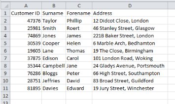
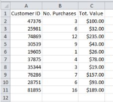
The tables below demonstrate a very simple example of a time when combining two tables might be useful. Both tables include the ‘Customer ID’ field, which can be used as the unique identifier, so combining them definitely possible.
The basic formula for using the VLOOKUP function is as follows:
=VLOOKUP(unique_identifier,lookup_table,column_index_number,range_lookup?)
I appreciate that this looks a bit complicated, but I promise it really isn’t! Here’s a quick explanation of the information Excel needs to process your formula:
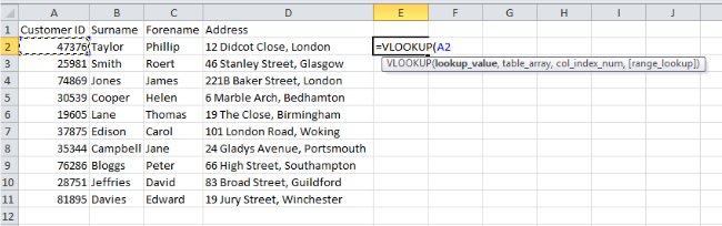
Unique identifier – This is the cell reference of the unique value that must appear in both of the tables. Usually you’ll use the VLOOKUP function at the end of a row in your primary table, so it’ll look something like this:
Lookup table – This is a cell range reference for the secondary table you’re using. It’s important to note that your secondary table should always have the unique identifier as its first column. If it doesn’t when you get your hands on it, just cut and paste the column you’ll be using as your unique identifier so that it’s the first column.
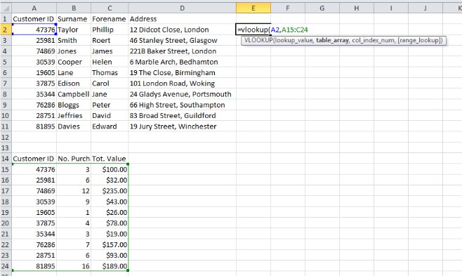
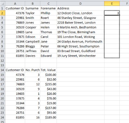
In the example below I’ve moved the secondary table so that it’s immediately below the primary table. In practice you probably won’t want to do this, I’ve done it purely so that it would fit into the screenshot.
Column index number – This is the number of the column within your secondary table that you want to bring into your primary table. Let’s say for now that I want to add the ‘No. Purchases’ column from the secondary table into the primary table – This is a second column in the table, so I’ll enter the number 2 into my formula. Note that the column index number has nothing to do with column or cell references, you simply need to count the number of columns.
Range lookup? – This is probably the least well understood aspect of the VLOOKUP function, but it’s actually quite simple. Essentially what you’re being asked is whether you want to bring back exact matches only, or whether you want to return any values falling within a specified range. I’ll come back to this later to explain further, but for now we are only looking for exact matches so we’re going to type FALSE into our formula.
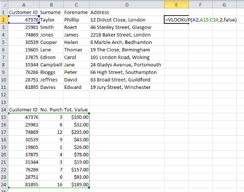
So now our formula is as follows: =VLOOKUP(A2,A15:C24,2,FALSE)
Most of the time when you’re using this function you’ll want to use it in each row of a large data table. That’s certainly true in this example so we’re going to want to copy the formula we’ve just written down using the Autofill Function so that it performs the same function for each customer record. Before we copy the formula down, though, we’re going to need to make a small change. When you use Autofill to copy a formula down to multiple rows Excel automatically updates the cell reference for you – That great because the unique identifier for each customer record will be different, but what about the secondary table? We’ve entered a specific cell range reference, and we want to use it for every row.
In order to achieve this we’ll need to add dollar signs to before the column and row number in each cell reference that we want to stop Excel from altering. In this example that’s going to look like this:
=VLOOKUP(A2,$A$15:$C$24,2,FALSE)
When you add dollar signs to a cell reference like this it is known as an Absolute Reference.
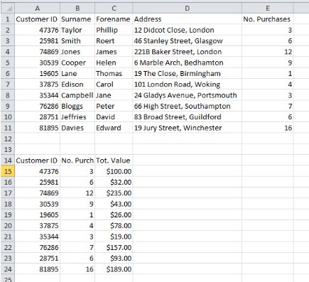
Once you’ve copied the formula down to all of the rows of your primary table, you can simply add the column header and you have successfully added the extra column to your data.
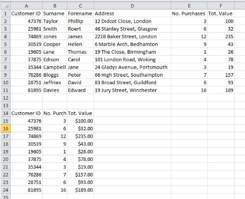
What if we wanted to add the ‘Tot. Value’ data to our primary data table as well? Easy, we can even use the formula we’ve already written, with one small change. The ‘Tot. Value’ column is the third column of data in our secondary table, so our formula will become: =VLOOKUP(A2,$A$15:$C$24,3,FALSE)
By following the same process we used for the first formula we can quickly add the ‘Tot. Value’ column to our primary data table:
And there we have it – A completed primary data table. I hope that this tutorial will help you to add this Excel function to your vocabulary, as it’s probably saved me more time than any other tool. Used properly this function can help you to do work in minutes that would otherwise have taken hours or days. The example I’ve used here is very simple and could easily have been done without using this function, but in my working life I have had to do similar merges with data tables that ran to more than 50,000 rows. Imagine doing that manually!
Range Lookups
Before I bring this tutorial to a close, I promised that I would give an explanation of the ‘Range Lookup?’ part of the VLOOKUP formula. Answering TRUE to this part of the formula will tell Excel that the data in your unique identifier column does not need to match the data in the secondary data table precisely, it can instead fall within a range. This is extremely useful when you’re analysing data, as it allows you to quickly group rows into various categories. In the screenshot below I’ve added an age column to our basic primary dataset, and I’m using the VLOOKUP function to organise the customer records into age brackets.
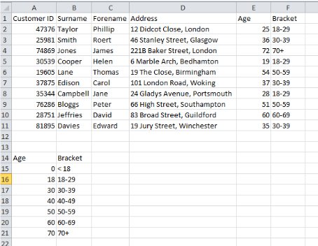
The formula I’ve used in cell F2 is: =VLOOKUP(E2,$A$15:$B$21,2,TRUE)
If you want to use the Range Lookup part of the VLOOKUP function you’re going to have to make your own secondary data table, which is exactly what I’ve done here. In the first column I’ve entered the first age that I want to fall into each bracket, and in the second column I’ve entered the text I want to add to the primary data table for any customers that fall between that age and the next one.
Essentially when you’re constructing a Range Lookup table you need to start each new row with the lowest value you want to fall into that bracket. In this instance, I want anyone under the age of 18 to be labelled as ‘<18’, anyone between the ages of 18 and 29 to be labelled as ’18-29’, and so on.
Once you’ve completed an exercise like this you’ll find that it’s much easier to use filters and charts to analyse your data in a logical way.
If you’re still struggling with the VLOOKUP Function you might find it helpful to have another look at the Getting started with Excel formulas page.
Looking for more? Return to Excel Formulas or the Office Software homepage


