Conditional Formatting
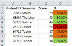
By using conditional formatting you can ask Excel to make various cosmetic changes to a cell or ranges of cells depending on their contents. For example, if you were working with test results, you could use conditional formatting to colour the cells containing the results green, orange or red dependent on each student’s score.
This is a function that has seen significant developments in later versions of Excel. In earlier versions, namely Excel 2003 and before, it was possible to add a maximum of 3 ‘conditions’ or ‘rules’ to any given cell. In practice this meant that it was possible to use a colour code which included 4 colours, as the cells being formatted could have a base colour which would then be altered by the conditional formatting.
From Excel 2007 onwards significant additional development has occurred, meaning that it’s now possible to add as many conditions as you like to any given cell. In addition to this the newer versions include a number of pre-set symbol systems which can automatically add traffic lights, coloured arrows, flags etc. to the cells depending on your defined conditions. Finally the process of creating new rules had been significantly simplified, which has the result of removing the need in many cases to use formulas to achieve your desired result.
So how does it work? Well, I’ll split this explanation down the middle and explain the two different versions of events separately – Click the following links to skip to the relevant explanation:
Basic explanation based on Excel 2003 and earlier
Excel 2007 and later - Developments
Excel 2003 and earlier
You can find the conditional formatting options in the ‘Formatting’ menu on the toolbar. Once you’ve selected it you’ll have a screen that looks something like this:
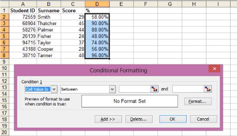
At this point you can choose between ‘Cell Value Is’, which will take you down the route selecting from various other menus in order to help setup your first condition, or you can select ‘Formula Is’. If you select the formula option you can use any Excel formula which will return a TRUE or FALSE value.
Click here for more information about Excel Formulas
If you go down the ‘Cell Value Is’ route, you can select from various options:
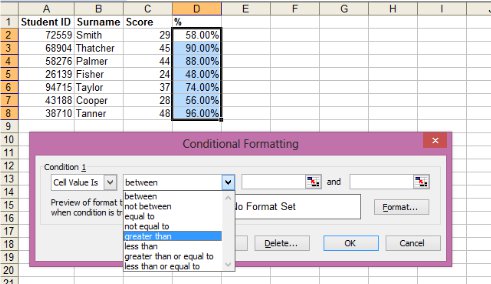
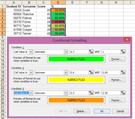
If you simply want to colour cells based on a single condition you can simply select one of these options, enter values or cell references into the next section and then move on to your choice of formatting. Here is an example of what that might look like:
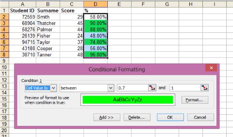
Note that in practice your conditions will not be applied until after you have clicked the ‘OK’ button, I’ve re-opened the options menu in the above screenshot so that you can see both the conditions I’ve set and their result on my selected cells. Also note that when working with percentages it’s important to remember that 100% is actually equal to 1, not 100, so you will need to divide any percentage figures by 100 when entering them as conditions. For example in this case 70% becomes 0.7.
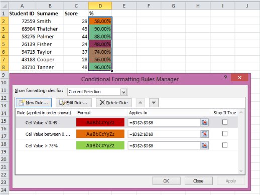
In practice you’ll probably find that you want to apply several conditions to your selected cells, so that it is easy to see how they compare to each other. In this example I’ve set 3 conditions, and I also started the process by colouring all of the cells in red with normal formatting options. This allows me to use a 4 colour code, even though I’m only able to set 3 conditions.
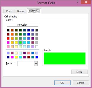
To set the formatting options for each condition, simply click on the ‘Format…’ button and you’ll see the following menu – You’ll be able to make changes to borders, shading, fonts, etc.
So that’s about it, now we’re on to…
Excel 2007 and later
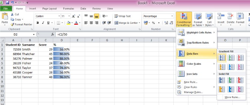
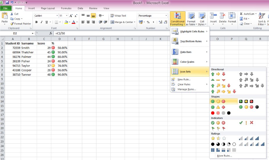
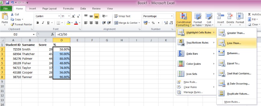
In later versions of Excel the Conditional Formatting menu can be found on the ‘Home’ tab on the ribbon. The options menu now takes the form of an interactive drop-down list, which contains a large number of pre-set options. These new options include data bars, traffic lights, colour scales and more. Here are a couple of examples:
And of course you can still set rules the old fashioned way by selecting the ‘Manage Rules’ option. This will allow you to see precisely what conditions have been set either by yourself or by using the pre-set options displayed above.
If you want to create a new rule from scratch you have two options – Select an option from ‘Highlight Cells Rules’ or ‘Top/Bottom Rules’, or use the ‘New Rule’ menu. All of these options can be reached from the main Conditional Formatting drop-down.
If you take the first route you’ll have a wide variety of options to choose from, which will meet the vast majority of needs.
Once you’ve selected the option you want you can simply enter the parameters of your condition and select the formatting options you want as normal.
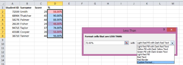
Choosing the ‘Custom Format…’ option will allow you to make formatting choices with the standard formatting menu.
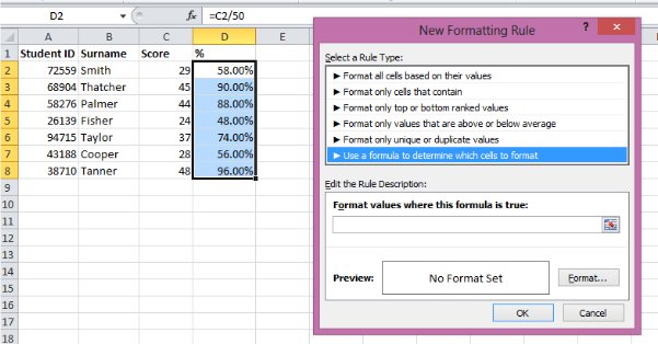
If you want to use a formula in your condition you will need to use the ‘New Rule’ menu – This can be reached either from the ‘Manage Rules’ menu, or from the main Conditional Formatting drop-down. Once you have the ‘New Formatting Rule’ menu up, simple select the formula options and proceed as normal to use any Excel Formula which will result in a TRUE or FALSE value.
Click here for more information about Excel Formulas
From the ‘New Rule’ menu you are still able to create new conditions using standard arguments if you wish, although it’s generally easier to use the first method I described above for these occasions.
So that’s all for this Conditional Formatting Tutorial, I hope you’ve found it helpful. Please let me know your thoughts by completing the feedback form at the bottom of the page.
Looking for more? Return to Excel Tutorials or the Office Software homepage


