Excel Drop Down Lists
Excel drop down lists are very useful if you’re creating data entry forms or other spreadsheets designed for use by multiple people. Adding a drop down list to a cell is a great way to force users of your spreadsheet to select certain pre-set values rather than whatever they’re thinking at the time – Very useful when collecting large volumes of data.
In order to add an Excel drop down list you’ll need to select the cell or cells you want to add the drop down list to and use the ‘Data Validation’ menu. In Excel 2003 or earlier you can reach this by selecting the ‘Data’ menu and then clicking on ‘Validation’, and in Excel 2007 or later you’ll need to select the ‘Data’ tab in the ribbon, click on the ‘Data Validation’ drop down and then select ‘Data Validation…’.
Regardless of which version you’re using, you’ll be greeted with a menu that looks like this –
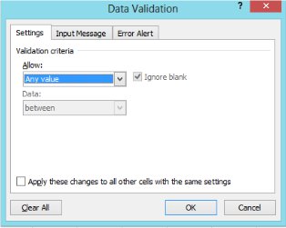
In the ‘Allow’ box you’ll need to select ‘List’ which will introduce a new options box called ‘Source’. It is at this point in the process that you’ll tell Excel what options you want to include in your dropdown list, and for that you have 3 options.
Type your options directly into the 'Source' box, separated by commas
For example if you want your Excel drop down list to include the numbers one to five, you would type the following: 1,2,3,4,5
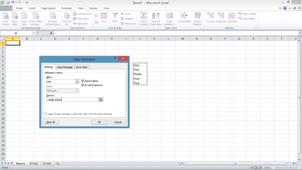
Type in or select a range of cells which contain your list of options
Most likely it will be convenient to select your cell range rather than typing it in – To do this simply click the ‘Cell Select’ button to the right of the ‘Source’ box and then select the range of cells you want to use.
Use a named range of cells
I’m not going to go too deeply into named ranges for the purposes of this tutorial, but it will sometimes be convenient for you to use a range of cells for your Excel drop down list. The ‘List’ data validation function has a minor limitation which will prevent you from selecting a range of cells that are situated in a different tab. The ‘get around’ for this limitation is to name the range of cells in question, and then enter ‘=NAME’ into the source box.
To name a range of cells simply exit the ‘Data Validation’ menu, and select the range as normal. You can now name this range by typing into the ‘Name Box’ which is situated on the menu bar or ribbon just above the cell A1. You can type whatever you want into this box provided that there are no spaces and you stick to simple symbols such as hyphens or underscores. Before you start typing into the ‘Name Box’ it will contain a cell reference – This can be safely overtyped. Here’s an example:
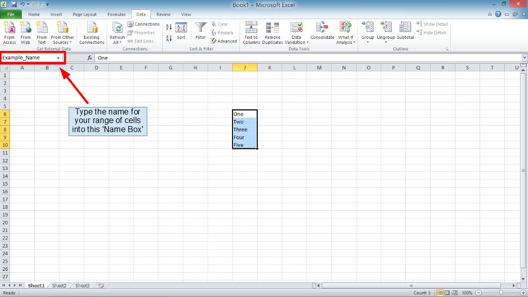
In this case I’ve named my range ‘Example_Name’, so I’ll type the following into the ‘Source’ box in the ‘Data Validation’ menu: =Example_Name
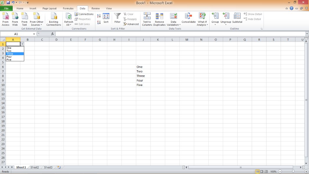
The Result
Regardless of which method you used for entering the desired options for your Excel drop down list, the result will be the same. Simply click the OK button to complete your data validation options, and the drop down list will be created. If you now select the cell or cells which you’ve added the drop down list to, you’ll find that it now has a down pointing arrow next to it. If you click on that arrow you’ll now be able to select one of the options you’ve just added to the ‘Data Validation’ menu.
If at any point you want to remove the Excel drop down list, simply select the cell or cells in question and return to the ‘Data Validation’ menu. In the ‘Allow’ box select ‘Any Value’ to remove your data validation options and return the cells to their normal state.
So that’s all for this Excel Drop Down List Tutorial, I hope you’ve found it helpful. Please let me know your thoughts by completing the feedback form at the bottom of the page.
Looking for more? Return to Excel Tutorials or the Office Software homepage


